
Making a map
A map is a time-series of stacks. You create a map by appending stacks from the stack browser. Once a map is made it can be saved, re-opened, annotated, and browsed using the time-series panel.
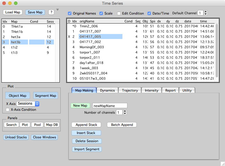
The time-series panel shows a list of open maps on the left. When a map is selected (het3b in this example), a list of sessions in the map are shown on the right (in this example there are 12 sessions).
1. Pre-process your raw data
Map Manager is designed to import single channel .tif stacks in a particular format. If your stacks have been acquired with proprietary software such as Zeiss Zen, Scan Image, Prairie View, or Nikon nd2 (Olympus coming soon) they need to be converted into a format for import into Map Manager.
We have Fiji plugins to do exactly this for Zeiss LSM/CZI, Prairie View, ScanImage, and Nikon nd2 files.
- Zeiss LSM/CZI, use bFolder2MapManager
- ScanImage, use bFolder2MapManager
- Nikon nd2, use bFolder2MapManager
- Prairie View, use bPrairie2tif
Please note, there does not seem to be date/time information in Nikon nd2 files. If anyone has more insight into this, please cantact robert.cudmore@gmail.com.
2. Open and initialize Map Manager
- Open Igor Pro with the provided MapManager .ipf file. This will look something like ‘MapManager_20180810.ipf’ where 20180810 is the release date of Map Manager.
- Click on the empty command window to activate Map Manager and its menus. If that does not work, click the ‘compile’ button in the opened source code window.
- Open the stack browser window with menu ‘MapManager - Stack Browser’.
- Open the time-series window with menu ‘MapManager - Time series’.
3. Make a new map
In the time-series window ‘Map Making’ tab
- Enter a new map name.
- Set the number of color channels for the map.
- Create a new map with the ‘New Map’ button.
Tip. It is important to specify the number of color channels in new maps with 'number of color channels'.
3.1 Appending stacks to your map
- In the stack browser, select the stack to be appended to the map.
- In the time-series panel ‘Map Making’ tab, press ‘Append Stack’ button.
- Repeat for each stack to be appended to the map.
Important
- Number of channels is important. When making a new map, you need to choose the ‘Number Of Color Channels’ properly. Map Manager will only allow one choice of ‘Number Of Color Channels’ per map. You cannot mix stacks with different numbers of channels within a map.
- Stack scale is important. Make sure the scale of each imported stack is correct. It is hard to change the scale later. If you use the provided Fiji plugins this should be taken care of. If necessary, set the scale of a stack in its stack window with shift+p BEFORE MAKING ANNOTATIONS.
- The order of stacks is important. Make sure the timepoints in your map are imported in the correct order. It is hard to change the order later.
3.2 Saving a map
Save the map with ‘Save Map’ button. New maps are saved to a default hard-drive folder specified in the Hard Drive Paths panel.
3.3 Opening a map
Open a previously saved Map Manager map using the ‘Open Map’ button in the time-series panel. When you open a map named ‘mymap’, you need to open the file ‘mymap.ipf’.
3.4 Congratulations, you just made a Map Manager map.
The rest of this workflow covers tracing dendritic segments, adding spines, and connecting spines across timepoints. Before you do any of this, play with the stacks in your map. From the time-series window, open a run of stacks by right-clicking on a session and selecting ‘Plot Run +- 1’.
4. Create dendritic tracings (for spine annotations)
All spine annotations are connected to a dendritic tracing. Dendritic tracings are first specified with control points annotations (In Map Manager) and then fit using a customized version of the Fiji plugin Simple-Neurite-Tracer. Before fitting a dendrite/segment in Fiji, you need to specify the path to a Fiji application in the Hard Drive Paths panel.
- Open a stack window. In the time-series panel, double-click the first session in your map.
- Create a line segment. See instruction in stack annotations ‘Creating and editing line segments’.
- Turn on the ‘Segment’ edit checkbox.
- Click the ‘+’ button to create a new (empty) segment.
- Create ‘Control Point’ annotations along a segment with shift+click. All points are in 3D, make sure the control points are in the center of the segment and in the correct imaging plane. If a control point is in complete darkness, the segment fitting in Fiji Simple-Neurite-Tracer will never find find a line (will never finish). Make sure your control points follow the segment in a linear fashion, you do not want to double back in the opposite direction.
- Delete control points with right-click menu ‘Delete’.
- Move control points with right-click menu ‘Move’.
- Once control points are made, fit the backbone line in Fiji. Right-click on your segment in the annotation control bar and select ‘Make from control points - Fiji’.
- Repeat steps # 1 and # 2 for each session in your map. Making the same line segment in each session. As you make control points, be sure they are in the same direction along the segment for each session.
- Set a pivot point in each line segment. Click a point in the segment, right-click and select ‘Set As Segment Pivot’.
Segment Pivot Points. The user specified segment pivot point in each segment should correspond to the same region of the segment across all time-points (sessions). A good strategy is to choose a region of the segment near an obvious spine that is present in all time-points (sessions). Another strategy is to choose a pivot point where some other segment (dendrite) crosses near your segment as these tend to remain stable across time. Try and put the pivot point near the center of the segment, do not place it at either the very beginning or the very end of a segment. The segment pivot point is used to calculate a line distance along the segment (in um) which in turn will be used to auto-guess corresponding spines between sessions.
Tip. When specifying control points and setting segment pivots, you can open multiple stack windows at the same time. Just double-click on each session in the time-series panel. This way, you can see the line segments you are making in each session of your map and make sure segment pivot points correspond to the same region of the dendrite/segment between time-points.
5. Connect line segments together (for spine annotations)
- Close all stack windows using the ‘Close Windows’ button in the time-series panel or use the main Map Manager menu - Close All Plots.
- Open a new stack run by right-clicking a session in your map (in the Time-series window) and selecting the ‘Plot Run +- All’ menu.
- Turn on the ‘Segments’ edit checkbox in the annotation control bar of a stack window. Open the annotation control bar with keyboard [.
- Sequentialy connect your line segment from one timepoint to the next
- Select the source timepoint segment (for example, timepoint 1). Make sure you select a point on the segment backbone line.
- Select the destination timepoint segment (for example, timepoint 2). Again, make sure you select a point on the segment backbone line.
- In the destination timepoint window (e.g. timepoint 2), press keyboard p for persistent or use right-click menu ‘Dynamics - Make Object Persistent’.
What have we done here? We have connected line segment tracings from one time-point to the next. This is neccessary because Map Manager allows you to have multiple line sgment tracings per stack and per time-point. We need to specify which line segment tracing corresponds to which line segment tracing between time-points. It is possible to have a dangling segment, for example, a segment that is traced in one time-point but not others.
Tip. Line segment tracings should always correspond to the same segment visualized across multiple time-points.
6. Create and edit annotations in each timepoint
Map Manager has two types of annotations: spines and other. A global option needs to be set to work with one or the other
- Open the global options panel with ‘MapManager - Options’.
- For spines, select ‘spines’ in the ‘Default scoring’ popup.
- For other, select ‘Cell Bodies’ in the ‘Default scoring’ popup.
All annotations are in 3D points, take care in creating the annotation in the correct image plane. See stack annotations for more detailed instructions.
Spines should be marked at the membrane limit of the spine head, somewhere near the tip of the spine.
6.1 Creating annotations
- Open a single timepoint stack window by double clicking a time-point (session) in the time-series window.
- Make sure ‘Segments’ edit checkbox is off. The segments ‘edit’ checkbox is in the annotation (left) control bar that is opened with keyboard ‘[’.
- For spines, select the segment to add a spine to by selecting it in the list of segments or single click a point along the segment tracing (in the image).
- Create an annotation with shift+click.
6.2 Editing annotations
- Select an annotation with a single-click, selected annotations appear yellow.
- Move an annotion with right-click ‘Move’.
- Delete an annotation with right-click ‘Delete’ or keyboard delete.
- Spines are automatically connected to the dendritic segment with a line. Edit the connection point with right-click ‘Manual Connect’ and then single-click the new connection point on the segment line.
6.3 Marking annotations bad
Be very liberal in your scoring, mark anything you think might be an annotation. Annotations can be flagged as ‘bad’ using the right-click menu ‘bad’. Bad annotations remain in the database but are not included in output reports. As your datasets grow, marking questionable annotations and then as bad allows you to return to a given image stack and see you already decided not to include a putative annotation in your analysis.
- Select an annotation with a single mouse click (selected annotations are yellow).
- Right-click and select ‘bad’
7. Edit the dynamics of annotations between timepoints
This is the core of Map Manager and you will spend most of your time doing this.
7.1 Manually specifying pivot points
Pivot points tell Map Manager how to snap images between time-point in a run plot and allow for automatic connections to be generated. The quality of the automatic connection will depend on the accuracy of manually specified pivot points.
Pivot points should correspond to a region of the image that is easily identifiable between timepoints. For spines, this would correspond to a large persistent spine, for other (Cell bodies) this would correspond to a stable cell body.
Pivot points for spine annotations are a point along the segment tracing. Right-click a point on the tracing line and select ‘Set as Segment Pivot’. This needs to be done for each segment in each time-point.
Pivot points for other(cell body) annotations are existing annotations flagged as a pivot. Right-click and existing annotation and select ‘Set as map pivot’. For pivot points to work, the annotation flagged as a pivot needs to first be connected through the map as persistent. Briefly: (1) select the annotation in the source timepoint, (2) select the desired annotation in the destination timepoint, (3) in the destination timepoint, press keyboard p.
7.2 Automatically connect annotations between time-points
- Open a map window with ‘Object Map’ button in the time-series panel.
- Single-click an annotation in the desired time-point (selected annotations appear yellow).
- Right-click and select menu ‘Dynamics - Connect objects to next’.
Automatic connections between time-points relies on manually specified pivot points. If pivot point are not specified or are poorly specified, automatic connections will not work.
7.3 Editing annotation dynamics manually from a run plot
Opening a run plot
- Open an object map from the time-series panel ‘Object Map’ button
- In the object map, right-click an annotation and select ‘Plot Run +- 1’. This will open a run plot which is a series of stack windows, one time-point per window.
- In a stack window in the run, control+click an annotation to snap all stacks in the run to the same image position. This will also automatically select all annotations that are persistent with the one you control+clicked.
- Once a spine is selected, use ctrl+left arrow and ctrl+right arrow to select the next spine along the tracing. As you do this, the other stack windows in the run will snap to the same image position and automatically select spines that have been marked as persistent.
Editing dynamics in a run plot
- Mark an annotation as addition. Select the annotation and press keyboard a.
- Mark an annotation as subtraction. Select the annotation and press keyboard s.
- Mark two annotations as persistent. Select the annotation in the source timepoint, then select the desired annotation in the destination timepoint. In the destination timepoint, press keyboard p.
As you edit the dynamics between annotations, all connections are automatically maintained. For example, marking an annotation as addition will automatically disconnect it from any previous annotation it was marked as persistent with.
New annotation are not connected to other time-points and are thus always both added and subtracted (e.g. transient). Annotations in the first timepoint can never be marked as added or transient. Likewise, annotations in the final timepoint can never be marked as subtraction or transient.
7.4 Editing annotation dynamics with Find Points
The dynamics of annotations can be edited using the Find Points panel. This is done pair-wise between timepoints. For example, if your map has 4 sessions, you will use Find Points first between session 1 and 2, then between sessions 2 and 3, and finally between sessions 3 and 4.
The Find Points panel will generate an automatic guess for the best connections and allow you to set them manually. This automatic guess is using the pivot point in your dendritic segment, if this pivot point does not correspond to a similar region of the segment between timepoints, the guess will be incorrect.
- Close all stack windows with ‘Close Windows’ button in time-series panel.
- Open the Find Points panel by right-clicking the first session in your map and selecting ‘Find Points’.
- In the Find Points panel, you are given a list of all annotations in the source timepoint. Click on an annotation in the list and Find Points will open both the source and destination timepoints, zoomed onto that annotation.
8. Curating your connected objects
8.1 Review your work by using search to query all addition, subtraction and transient
- Open the search panel from the time-series panel with the ‘Search’ button.
- Search for added annotations with the ‘Addition’ button. The ‘Addition’ button is in the ‘Map’ tab.
- All added annotations will appear as a list in the search results.
- Right-click on an annotation and select ‘plot run +- 1’ to bring up a spine run.
- Visually check that you agree the annotation is an addition and edit if necessary. Once you are in a run plot, you can always add and delete annotations, and edit the dynamics manually.
- Do the same by searching for ‘Subtraction’ and then ‘Transient’
8.2 Browse the connections visually and edit as necessary
This is a repeat of what we already described above
You need to verify the connectivity of annotations between all timepoints in the map. If your map has 4 timepoints, you need to verify the annotation connections between timepoint 1-2, timepoint 2-3, and timepoint 3-4.
- Open a run plot of three sequential timepoints by right-clicking a spine in the object map and selecting ‘plot run +- 1’. Open an object map with the ‘Object Map’ button in the time-series panel.
- In the run plot windows, select an annotation in the middle timepoint with ctrl+click. This will snap and zoom the annotations and its associated connections in all windows of the run plot. If there is no annotation in a given timepoint, the image will be snapped to where the annotation ‘would-be’. This is using segment pivot points, if they are not specified or poorly marked, this snapping will not work.
- From the middle timepoint spine selection, go to the next spine along the segment using keyboard ctrl+right arrow. Go to the previous spine along the segment using keyboard ctrl+left arrow.
- Correct any errors in the spine dynamics using keyboard a for addition, s for subtraction, and p for persistence. See run plot for details.